
 RSS
RSSLog normal distribution
Where do you meet this distribution?
- Finance, Economics : Change of stock price
Shape of Distribution
Basic Properties
- Two parameters
are required (How can you get these).
- Continuous distribution defined on semi-bounded range
- This distribution is always asymmetric.


Probability
- Cumulative distribution function
where
is cumulative distribution function of standard normal distribution.
- Probability density function
where
is probability density function of standard normal distribution.
- How to compute these on Excel.
1 2 3 4 5 6
7
A B Data Description 0.5 Value for which you want the distribution 0.1 Value of parameter M 2 Value of parameter S Formula Description (Result) =NTLOGNORMDIST(A2,A3,A4,TRUE) Cumulative distribution function for the terms above =NTLOGNORMDIST(A2,A3,A4,FALSE) Probability density function for the terms above 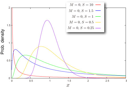
- Function reference : NTLOGNORMDIST
=\Phi\left(\frac{\ln x-M}{S}\right)")
=\frac{1}{Sx}\phi\left(\frac{\ln x-M}{S}\right)")
Quantile
- Inverse function of cumulative distribution function
where
- How to compute this on Excel.
1 2 3 4 5 6
A B Data Description 0.7 Probability associated with the distribution 0.1 Value of parameter M 2 Value of parameter S Formula Description (Result) =NTLOGNORMINV(A2,A3,A4) Inverse of the cumulative distribution function for the terms above
![F^{-1}(P)=\exp\left[S\Phi^{-1}(P)+M\right]](https://s0.wp.com/latex.php?latex=F%5E%7B-1%7D%28P%29%3D%5Cexp%5Cleft%5BS%5CPhi%5E%7B-1%7D%28P%29%2BM%5Cright%5D&bg=T&fg=000000&s=0 "F^{-1}(P)=\exp\left[S\Phi^{-1}(P)+M\right]")
Characteristics
Mean – Where is the “center” of the distribution? (Definition)
- Mean of the distribution is given as
where
- How to compute this on Excel
1 2 3 4 5 A B Data Description 0.1 Value of parameter M 2 Value of parameter S Formula Description (Result) =NTLOGNORMMEAN(A2,A3) Mean of the distribution for the terms above - Function reference : NTLOGNORMMEAN

,\;\omega=\exp(S^2)")
Standard Deviation – How wide does the distribution spread? (Definition)
- Variance of the distribution is given as
where
Standard Deviation is a positive square root of Variance.
- How to compute this on Excel
1 2 3 4 5
A B Data Description 0.1 Value of parameter M 2 Value of parameter S Formula Description (Result) =NTLOGNORMSTDEV(A2,A3) Standard deviation of the distribution for the terms above - Function reference : NTLOGNORMSTDEV
")
Skewness – Which side is the distribution distorted into? (Definition)
- Skewness of the distribution is given as
where
- How to compute this on Excel
1 2 3 4 5 A B Data Description 0.1 Value of parameter M 2 Value of parameter S Formula Description (Result) =NTLOGNORMSKEW(A2,A3) Skewness of the distribution for the terms above - Function reference : NTLOGNORMSKEW
\sqrt{\omega-1}")
")
Kurtosis – Sharp or Dull, consequently Fat Tail or Thin Tail (Definition)
- Kurtosis of the distribution is given as
where
- How to compute this on Excel
1 2 3 4 5 A B Data Description 0.1 Value of parameter M 2 Value of parameter S Formula Description (Result) =NTLOGNORMKURT(A2,A3) Kurtosis of the distribution for the terms above - Function reference : NTLOGNORMKURT

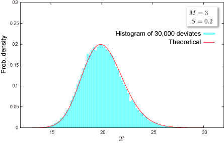
Random Numbers
- Random number x is generated by inverse function method, which is for uniform random U,
where
- How to generate random numbers on Excel.
1 2 3 4 5
A B Data Description 0.1 Value of parameter M 2 Value of parameter S Formula Description (Result) =NTRANDLOGNORM(100,A2,A3,0) 100 log normal deviates based on Mersenne-Twister algorithm for which the parameters above Note The formula in the example must be entered as an array formula. After copying the example to a blank worksheet, select the range A7:A106 starting with the formula cell. Press F2, and then press CTRL+SHIFT+ENTER.
- Function reference : NTRANDLOGNORM
![x=\exp\left[S\Phi^{-1}(U)+M\right]](https://s0.wp.com/latex.php?latex=x%3D%5Cexp%5Cleft%5BS%5CPhi%5E%7B-1%7D%28U%29%2BM%5Cright%5D&bg=T&fg=000000&s=0 "x=\exp\left[S\Phi^{-1}(U)+M\right]")
NtRand Functions
- If you already have parameters of the distribution
- Generating random numbers based on Mersenne Twister algorithm: NTRANDLOGNORM
- Computing probability : NTLOGNORMDIST
- Computing mean : NTLOGNORMMEAN
- Computing standard deviation : NTLOGNORMSTDEV
- Computing skewness : NTLOGNORMSKEW
- Computing kurtosis : NTLOGNORMKURT
- Computing moments above at once : NTLOGNORMMOM
- If you know mean and standard deviation of the distribution
- Estimating parameters of the distribution:NTLOGNORMPARAM
Reference
- Wolfram Mathworld – Log Normal Distribution
- Wikipedia – Log-normal distribution
- Statistics Online Computational Resource